Examples

Each script in examples/ is short and self-contained, and shows one idea. Run any of them from the project root:

python examples/identity/01_basic_interval.py

Note

The examples pass a short m_values range so most run in a few seconds. Make sure felcu is installed in editable mode (pip install -e .) so they use your working copy.

Identity

Identity on a symmetric interval

Fit \(f(\mathcal H) = \mathcal H\) for a Hermitian \(\mathcal H\) with eigenvalues in \([-1, 1]\).

felcu centres the fit at \(\mu = 0\), the middle of the interval, and fits \(g(x) = x/\tau\). Because that is odd, every cosine coefficient \(b_k\) and the constant term \(a_0\) vanish.

examples/identity/01_basic_interval.py

"""
Identity on a symmetric interval
================================

Fit f(H) = H for a Hermitian H with eigenvalues in [-1, 1].

felcu centres the fit at mu = 0, the middle of the interval, and fits
g(x) = x / tau.  Because that is odd, every cosine coefficient (bk) and
the constant term (a0) vanish.

Run with:
    python examples/identity/01_basic_interval.py
"""

import numpy as np

from felcu import solve_fe_coefficients

result = solve_fe_coefficients(
    "identity",
    sigma_min=-1.0,
    sigma_max=1.0,
    target_error=1e-8,
    m_values=range(4, 33, 2),  # short sweep for speed; default goes to m=256
)

print(f"converged      = {result.converged}")
print(f"basis          = {result.basis_used}")
print(f"m              = {result.m}")
print(f"tau            = {result.tau:.4f}   (fit g(x) = x / tau, then f(H) = g(tau H))")
print(f"Linf error     = {result.achieved_linf_error:.2e}")
print(f"alpha (LCU)    = {result.alpha:.4f}")
print(f"|a0|           = {abs(result.a0):.1e}")
print(f"max |bk|       = {np.max(np.abs(result.bk)):.1e}")
print(f"first 5 ak     = {np.array2string(result.ak[:5], precision=4)}")

Identity on an off-centre interval

For eigenvalues in \([2, 5]\), felcu centres the fit at \(\mu = 3.5\):

\[ g(x) = \mu + \frac{x}{\tau}, \qquad f(\mathcal H) = g(\tau(\mathcal H - \mu I)), \]

so the constant term carries \(\mu\) and only the half-width needs fitting.

\(\mathcal H\) is positive definite here, so its singular values are its eigenvalues, and spectral_kind='singular_values' fits them through the Hermitian dilation instead. The dilation's spectrum, \([-5, -2] \cup [2, 5]\), is centred at \(0\), so \(\mu = 0\) and the odd \(g(x) = x/\tau\) covers the whole of \([-5, 5]\), which costs a larger \(\alpha_m\).

examples/identity/02_off_centre.py

"""
Identity on an off-centre interval
==================================

For eigenvalues in [2, 5], felcu centres the fit at mu = 3.5:

    g(x) = mu + x / tau,   f(H) = g(tau (H - mu I))

so the constant term carries mu and only the half-width needs fitting.

H is positive definite here, so its singular values are its eigenvalues,
and spectral_kind='singular_values' fits them through the Hermitian
dilation instead.  The dilation's spectrum, [-5, -2] U [2, 5], is centred at
0, so mu = 0 and the odd g(x) = x / tau covers the whole of [-5, 5], which
costs a larger alpha.

Run with:
    python examples/identity/02_off_centre.py
"""

from felcu import solve_fe_coefficients

kwargs = dict(sigma_min=2.0, sigma_max=5.0, target_error=1e-8, m_values=range(4, 33, 2))

for kind in ("eigenvalues", "singular_values"):
    r = solve_fe_coefficients("identity", spectral_kind=kind, **kwargs)
    print(
        f"{kind:<15}  mu={r.mu:<4}  basis={r.basis_used:<16}  m={r.m:<4}  "
        f"a0={r.a0:.4f}  alpha={r.alpha:.4f}  Linf={r.achieved_linf_error:.1e}"
    )

Identity from a Hermitian matrix

Pass the matrix itself: felcu reads its eigenvalue range. We then check the block-encoded operator \(g(\tau(\mathcal H - \mu I))\) against \(\mathcal H\) using an eigendecomposition, with \(\mu\) the centre of the eigenvalue range.

examples/identity/03_hermitian_matrix.py

"""
Identity from a Hermitian matrix
================================

Pass the matrix itself: felcu reads its eigenvalue range.  We then check
the block-encoded operator g(tau (H - mu I)) against H using an
eigendecomposition, with mu the centre of the eigenvalue range.

Run with:
    python examples/identity/03_hermitian_matrix.py
"""

import numpy as np

from felcu import solve_fe_coefficients

rng = np.random.default_rng(0)
n = 8
X = rng.standard_normal((n, n)) + 1j * rng.standard_normal((n, n))
H = (X + X.conj().T) / 4  # random complex Hermitian

result = solve_fe_coefficients("identity", matrix=H, target_error=1e-8, m_values=range(4, 33, 2))
print(f"spectral kind   = {result.spectral_kind_used}")
print(f"eigenvalues in  = [{result.sigma_min:.4f}, {result.sigma_max:.4f}]")
print(f"mu              = {result.mu:.4f}")
print(f"m               = {result.m}")

H_approx = result.apply(H)  # g(tau (H - mu I)), by eigendecomposition

print(f"||g(tau (H - mu I)) - H||_2 = {np.linalg.norm(H_approx - H, 2):.2e}")

Identity on a non-Hermitian matrix

For a non-Hermitian \(A\), felcu switches to the singular values automatically. The odd sine series acts on the singular values (as in QSVT): with \(A = U\Sigma V^\dagger\),

\[ U g(\tau\Sigma) V^\dagger \approx A . \]

examples/identity/04_non_hermitian_matrix.py

"""
Identity on a non-Hermitian matrix
==================================

For a non-Hermitian A, felcu switches to the singular values automatically.
The odd sine series acts on the singular values (as in QSVT):

    g(tau A) = U diag(g(tau s)) V^dagger  ~=  A

result.evaluate(s) gives g(tau s) for the singular values s.

Run with:
    python examples/identity/04_non_hermitian_matrix.py
"""

import numpy as np

from felcu import solve_fe_coefficients

rng = np.random.default_rng(1)
A = rng.standard_normal((6, 6)) / 3

result = solve_fe_coefficients("identity", matrix=A, target_error=1e-8, m_values=range(4, 33, 2))
print(f"hermitian?           = {result.matrix_is_hermitian}")
print(f"spectral kind        = {result.spectral_kind_used}")
print(f"singular values in   = [{result.sigma_min:.4f}, {result.sigma_max:.4f}]")
print(f"m                    = {result.m}")

U, s, Vh = np.linalg.svd(A)
A_approx = U @ np.diag(result.evaluate(s)) @ Vh

print(f"||g(tau A) - A||_2   = {np.linalg.norm(A_approx - A, 2):.2e}")

Inversion

Inversion on a definite interval

Fit \(f(\mathcal H) = \mathcal H^{-1}\) for eigenvalues in \([0.5, 3]\).

The target \(1/x\) has a pole at \(0\). The interval is definite, so the pole lies outside it, and the default \(\eta\) places it on the periodic boundary, \(x = -\tau\mu = -\pi\).

examples/inversion/01_basic_interval.py

"""
Inversion on a definite interval
================================

Fit f(H) = H^{-1} for eigenvalues in [0.5, 3].

The target 1/x has a pole at 0.  The interval is definite, so the pole lies
outside it, and the default eta places it on the periodic boundary,
x = -tau mu = -pi.

Run with:
    python examples/inversion/01_basic_interval.py
"""

from felcu import solve_fe_coefficients

result = solve_fe_coefficients(
    "inversion",
    sigma_min=0.5,
    sigma_max=3.0,
    target_error=1e-6,
    m_values=range(4, 65, 4),  # short sweep for speed; default goes to m=256
)

print(f"converged   = {result.converged}")
print(f"mu, tau     = {result.mu:.4f}, {result.tau:.4f}")
print(f"pole at x   = {-result.tau * result.mu:.4f}")
print(f"basis       = {result.basis_used}")
print(f"eta         = {result.eta:.4f}   (default (kappa + 1) / (kappa - 1))")
print(f"m           = {result.m}")
print(f"Linf error  = {result.achieved_linf_error:.2e}")
print(f"alpha (LCU) = {result.alpha:.4f}")

Cost of inversion versus condition number

Fix \(\lambda_{\max} = 1\) (sigma_max) and shrink \(\lambda_{\min}\) (sigma_min), so the condition number \(\kappa = 1/\lambda_{\min}\) grows. Both the truncation order \(m\) and the subnormalisation \(\alpha_m\) increase.

examples/inversion/02_condition_number.py

"""
Cost of inversion versus condition number
=========================================

Fix sigma_max = 1 and shrink sigma_min, so kappa = 1 / sigma_min grows.
Both the truncation order m and the subnormalisation alpha increase.

Run with:
    python examples/inversion/02_condition_number.py
"""

from felcu import solve_fe_coefficients

print(f"{'kappa':>6}  {'m':>4}  {'alpha':>10}  {'Linf':>9}  converged")
for kappa in [2, 5, 10, 20]:
    r = solve_fe_coefficients(
        "inversion",
        sigma_min=1.0 / kappa,
        sigma_max=1.0,
        target_error=1e-4,
        m_values=range(4, 101, 4),  # short sweep for speed; default goes to m=256
        selection="smallest_m",  # report the shortest series that meets the target
    )
    print(f"{kappa:>6}  {r.m:>4}  {r.alpha:>10.3f}  {r.achieved_linf_error:>9.1e}  {r.converged}")

Inverting a non-Hermitian matrix

\(A\) has no real eigenvalue interval, so felcu fits its singular values, through the Hermitian dilation \(\mathcal H = \begin{pmatrix} 0 & A \\ A^\dagger & 0 \end{pmatrix}\). The dilation's spectrum is symmetric about \(0\), so \(\mu = 0\), and the fit is the odd \(g(x) = \tau/x\) on two intervals either side of the pole. With \(A = U\Sigma V^\dagger\),

\[ V g(\tau\Sigma) U^\dagger \approx A^{-1} . \]

examples/inversion/03_non_hermitian_matrix.py

"""
Inverting a non-Hermitian matrix
================================

A has no real eigenvalue interval, so felcu fits its singular values,
through the Hermitian dilation [[0, A], [A^dagger, 0]].  The dilation's
spectrum is symmetric about 0, so mu = 0, and the fit is the odd
g(x) = tau / x on two intervals either side of the pole.  With
A = U diag(s) V^dagger,

    V diag(g(tau s)) U^dagger  ~=  A^{-1}

result.evaluate(s) gives g(tau s) for the singular values s.

Run with:
    python examples/inversion/03_non_hermitian_matrix.py
"""

import numpy as np

from felcu import solve_fe_coefficients

rng = np.random.default_rng(2)
U0, _ = np.linalg.qr(rng.standard_normal((5, 5)))
V0, _ = np.linalg.qr(rng.standard_normal((5, 5)))
A = U0 @ np.diag([0.4, 0.7, 1.0, 1.5, 2.0]) @ V0.T  # kappa = 5

result = solve_fe_coefficients("inversion", matrix=A, target_error=1e-6, m_values=range(4, 65, 4))
print(f"spectral kind       = {result.spectral_kind_used}  (mu = {result.mu})")
print(f"singular values in  = [{result.sigma_min:.4f}, {result.sigma_max:.4f}]")
print(f"m                   = {result.m}")

U, s, Vh = np.linalg.svd(A)
A_inv_approx = Vh.T @ np.diag(result.evaluate(s)) @ U.T

A_inv = np.linalg.inv(A)
print(f"||approx - A^-1||_2 = {np.linalg.norm(A_inv_approx - A_inv, 2):.2e}")
print(f"||A approx - I||_2  = {np.linalg.norm(A @ A_inv_approx - np.eye(5), 2):.2e}")

Inversion of a definite Hermitian matrix

When \(\mathcal H\) is definite (all eigenvalues the same sign), felcu fits \(1/x\) on a single interval centred at \(\mu\):

\[ f(\mathcal H) = g(\tau(\mathcal H - \mu I)) . \]

This works for positive- and negative-definite \(\mathcal H\) alike.

examples/inversion/04_definite_matrix.py

"""
Inversion of a definite Hermitian matrix
========================================

When H is definite (all eigenvalues the same sign), felcu fits 1/x on a
single interval centred at mu:

    f(H) = g(tau (H - mu I))

This works for positive- and negative-definite H alike.

Run with:
    python examples/inversion/04_definite_matrix.py
"""

import numpy as np

from felcu import solve_fe_coefficients

rng = np.random.default_rng(3)
Q, _ = np.linalg.qr(rng.standard_normal((6, 6)))

for label, eigs in [("positive definite", np.linspace(0.5, 2.0, 6)), ("negative definite", np.linspace(-2.0, -0.5, 6))]:
    H = Q @ np.diag(eigs) @ Q.T
    r = solve_fe_coefficients("inversion", matrix=H, target_error=1e-6, m_values=range(4, 65, 4))

    err = np.linalg.norm(r.apply(H) - np.linalg.inv(H), 2)

    print(
        f"{label}:  mu={r.mu:+.2f}  basis={r.basis_used}  m={r.m}  alpha={r.alpha:.3f}  ||approx - H^-1||_2={err:.1e}"
    )

Inversion of an indefinite Hermitian matrix

When \(\mathcal H\) has eigenvalues on both sides of \(0\), in \([\lambda_{\min}, a] \cup [b, \lambda_{\max}]\) with \(a < 0 < b\), felcu fits \(1/x\) on both parts and leaves the gap \((a, b)\) around the pole free. The fit is still centred at the midpoint \(\mu\) of \([\lambda_{\min}, \lambda_{\max}]\), which need not be \(0\):

\[ f(\mathcal H) = g(\tau(\mathcal H - \mu I)) . \]

With a matrix, the gap is read from its eigenvalues; with bounds, pass gap=(a, b).

examples/inversion/05_indefinite_matrix.py

"""
Inversion of an indefinite Hermitian matrix
===========================================

When H has eigenvalues on both sides of 0, in [lambda_min, a] U [b, lambda_max]
with a < 0 < b, felcu fits 1/x on both parts and leaves the gap (a, b) around
the pole free.  The fit is still centred at the midpoint mu of
[lambda_min, lambda_max], which need not be 0:

    f(H) = g(tau (H - mu I))

With a matrix, the gap is read from its eigenvalues; with bounds, pass
gap=(a, b).

Run with:
    python examples/inversion/05_indefinite_matrix.py
"""

import numpy as np

from felcu import solve_fe_coefficients

rng = np.random.default_rng(4)
Q, _ = np.linalg.qr(rng.standard_normal((6, 6)))
H = Q @ np.diag([-2.0, -1.2, -0.5, 0.4, 1.6, 3.0]) @ Q.T

r = solve_fe_coefficients("inversion", matrix=H, target_error=1e-6, m_values=range(8, 129, 8))
print(f"spectrum    = [{r.sigma_min:.2f}, {r.gap[0]:.2f}] U [{r.gap[1]:.2f}, {r.sigma_max:.2f}]")
print(f"mu, tau     = {r.mu:.4f}, {r.tau:.4f}")
print(f"fitted on   = [{-r.x_max:.4f}, {r.x_gap[0]:.4f}] U [{r.x_gap[1]:.4f}, {r.x_max:.4f}]")
print(f"eta         = {r.eta:.4f}   (default 1 + (b - a) / (2 delta))")
print(f"m, alpha    = {r.m}, {r.alpha:.4f}")

print(f"||approx - H^-1||_2 = {np.linalg.norm(r.apply(H) - np.linalg.inv(H), 2):.1e}")

same = solve_fe_coefficients(
    "inversion", sigma_min=-2.0, sigma_max=3.0, gap=(-0.5, 0.4), target_error=1e-6, m_values=range(8, 129, 8)
)
print(f"from bounds: m={same.m}  alpha={same.alpha:.4f}")

Exponentiation

Truncation order versus target error

Tighten target_error and watch how the selected order \(m\) grows. For a smooth target like \(e^x\), \(m\) grows roughly logarithmically in \(1/\epsilon_{\rm t}\).

examples/exponentiation/01_target_sweep.py

"""
Truncation order versus target error
====================================

Tighten target_error and watch how the selected order m grows.  For a
smooth target like exp, m grows roughly logarithmically in 1/error.

Run with:
    python examples/exponentiation/01_target_sweep.py
"""

from felcu import solve_fe_coefficients

print(f"{'target':>8}  {'m':>4}  {'Linf':>9}  {'alpha':>8}")
for target in [1e-2, 1e-4, 1e-6, 1e-8, 1e-10, 1e-12]:
    r = solve_fe_coefficients(
        "exponentiation",
        sigma_min=0.1,
        sigma_max=2.0,
        target_error=target,
        m_values=range(4, 41, 2),  # short sweep for speed; default goes to m=256
        selection="smallest_m",  # report the shortest series that meets the target
    )
    print(f"{target:>8.0e}  {r.m:>4}  {r.achieved_linf_error:>9.1e}  {r.alpha:>8.4f}")

Matrix exponential from a Hermitian matrix

Fit \(e^{\mathcal H}\) from \(\mathcal H\) directly, then compare \(g(\tau(\mathcal H - \mu I))\) with the exact matrix exponential computed by eigendecomposition.

examples/exponentiation/02_matrix_exponential.py

"""
Matrix exponential from a Hermitian matrix
==========================================

Fit exp(H) from H directly, then compare g(tau (H - mu I)) with the exact
matrix exponential computed by eigendecomposition.

Run with:
    python examples/exponentiation/02_matrix_exponential.py
"""

import numpy as np

from felcu import solve_fe_coefficients

rng = np.random.default_rng(4)
n = 10
X = rng.standard_normal((n, n))
H = (X + X.T) / 6  # random real symmetric

result = solve_fe_coefficients("exponentiation", matrix=H, target_error=1e-8, m_values=range(4, 33, 2))
print(f"eigenvalues in = [{result.sigma_min:.4f}, {result.sigma_max:.4f}]")
print(f"m              = {result.m}")

w, V = np.linalg.eigh(H)
exp_H = V @ np.diag(np.exp(w)) @ V.T
approx = result.apply(H)  # g(tau (H - mu I)), by eigendecomposition

print(f"||g(tau (H - mu I)) - exp(H)||_2 = {np.linalg.norm(approx - exp_H, 2):.2e}")

Complex coefficients for an LCU circuit

An LCU circuit implements \(\sum_k c_k e^{ikx}\). felcu returns these as result.complex_coefficients \(= [c_{-m}, \dots, c_0, \dots, c_m]\). The LCU subnormalisation \(\alpha_m = \sum_k |c_k|\) is the sum of their magnitudes. The example ends by printing the same coefficients as result.circuit_coefficients \(= [c_0, 0, c_1, c_{-1}, \dots, c_m, c_{-m}]\), the order the compressed circuit uses (the zero is required by it), then as a bare Python list for pasting by hand: complex_coefficients is ordered by \(k\) for evaluating the series, circuit_coefficients is what you pass to the circuit.

examples/exponentiation/03_lcu_coefficients.py

"""
Complex coefficients for an LCU circuit
=======================================

An LCU circuit implements sum_k c_k e^{i k x}.  felcu gives the same c_k in
two orders:

    result.complex_coefficients = [c_{-m}, ..., c_0, ..., c_m]
        ordered by k: use it to evaluate or analyse the series.  This is the
        order stored by to_json().

    result.circuit_coefficients = [c_0, 0, c_1, c_{-1}, ..., c_m, c_{-m}]
        the order the compressed circuit consumes them in: pass this one to
        the circuit.  The extra zero is required by the compressed circuit,
        so it has 2m + 2 entries.

Circuit code that imports felcu should take result.circuit_coefficients
directly.  To paste the coefficients by hand, print
result.format_circuit_coefficients(), a bare Python list that keeps the
zero after c_0.  The LCU subnormalisation alpha is the sum of the
magnitudes |c_k|, the same in either order.

Run with:
    python examples/exponentiation/03_lcu_coefficients.py
"""

import numpy as np

from felcu import solve_fe_coefficients

result = solve_fe_coefficients(
    "exponentiation",
    sigma_min=-1.0,
    sigma_max=1.0,
    target_error=1e-6,
    m_values=range(4, 33, 2),  # short sweep for speed; default goes to m=256
)
c = result.complex_coefficients
m = result.m

print(f"m = {m},  len(c) = {len(c)}  (= 2m + 1)")
print(f"{'k':>4}  {'|c_k|':>10}")
for k, ck in zip(range(-m, m + 1), c):
    print(f"{k:>4}  {abs(ck):>10.2e}")

# Evaluate the exponential form at a point and compare with exp(mu + x / tau)
mu = 0.5 * (result.sigma_min + result.sigma_max)
x = 0.3
g = np.sum(c * np.exp(1j * np.arange(-m, m + 1) * x))
print(f"\nsum c_k e^(ikx) at x={x}: {g.real:.8f}   (imag {g.imag:.1e})")
print(f"exp(mu + x / tau):         {np.exp(mu + x / result.tau):.8f}")
print(f"alpha = {result.alpha:.6f}")

# The same coefficients in circuit order: what circuit code should consume
cc = result.circuit_coefficients
print(f"\nlen(circuit_coefficients) = {len(cc)}  (= 2m + 2, with a zero after c_0)")
print(f"sum |c_k| in circuit order = {np.sum(np.abs(cc)):.6f}  (= alpha)")

# ... and as a bare list to paste by hand.  Keep the zero after c_0: the
# compressed circuit requires it.
print("\nCircuit order [c_0, 0, c_1, c_-1, ..., c_m, c_-m]; the zero after c_0 is required by the compressed circuit:")
print(result.format_circuit_coefficients())

Effect of the Sobolev regulariser

At fixed \(m\), felcu regularises with the \(H_r^w\) norm, weighting the \(k\)-th Fourier mode by \(P_w(r|k|) = \sum_{j=0}^{w} (r|k|)^{2j}\), and picks the largest regularisation weight \(\gamma\) that still meets target_error. Vary the order \(w\) and the scale \(r\) and see how lambda_used (\(= \sqrt{2\pi\gamma}\)) and the subnormalisation \(\alpha_m\) change.

examples/exponentiation/04_sobolev_regularisation.py

"""
Effect of the Sobolev regulariser
=================================

At fixed m, felcu regularises with the H_r^w norm, weighting the k-th
Fourier mode by 1 + (r|k|)^(2w), and picks the largest regularisation
weight that still meets target_error.  Vary the order w and the scale r
and see how lambda_used (= sqrt(2 pi gamma)) and the subnormalisation
alpha change.

Run with:
    python examples/exponentiation/04_sobolev_regularisation.py
"""

from felcu import solve_fe_coefficients

common = dict(sigma_min=0.1, sigma_max=2.0, target_error=1e-6, m=40)

print("Varying the order w (r = 1):")
for w in (0.75, 1.0, 1.5, 2.0):
    r = solve_fe_coefficients("exponentiation", sobolev_w=w, sobolev_r=1.0, **common)
    print(f"  w={w:<4}  lambda={r.lambda_used:.1e}  alpha={r.alpha:.6f}  Linf={r.achieved_linf_error:.1e}")

print("\nVarying the scale r (w = 1):")
for scale in (0.1, 0.25, 0.5, 1.0):
    r = solve_fe_coefficients("exponentiation", sobolev_w=1.0, sobolev_r=scale, **common)
    print(f"  r={scale:<4}  lambda={r.lambda_used:.1e}  alpha={r.alpha:.6f}  Linf={r.achieved_linf_error:.1e}")

Choosing between candidate truncation orders

With the default selection='smallest_alpha', felcu solves for every \(m\) in m_values, keeps all candidates in result.all_results, and picks the one with the smallest subnormalisation \(\alpha_m\). 'smallest_m' picks the shortest series that meets the target instead, and stops the sweep there.

examples/exponentiation/05_selection_and_candidates.py

"""
Choosing between candidate truncation orders
============================================

With the default selection='smallest_alpha', felcu solves for every m in
m_values, keeps all candidates in result.all_results, and picks the one
with the smallest subnormalisation.  'smallest_m' picks the shortest
series that meets the target instead, and stops the sweep there.

Run with:
    python examples/exponentiation/05_selection_and_candidates.py
"""

from felcu import solve_fe_coefficients

common = dict(sigma_min=0.1, sigma_max=2.0, target_error=1e-8, m_values=range(8, 41, 4))

r = solve_fe_coefficients("exponentiation", **common)
print(f"{'m':>4}  {'Linf':>9}  {'alpha':>9}  converged")
for c in r.all_results:
    print(f"{c.m:>4}  {c.achieved_linf_error:>9.1e}  {c.alpha:>9.6f}  {c.converged}")

for selection in ("smallest_m", "smallest_alpha"):
    s = solve_fe_coefficients("exponentiation", selection=selection, **common)
    print(f"\nselection={selection!r:<17} -> m={s.m}, alpha={s.alpha:.6f}")

Square root

Square root on a positive-definite interval

Fit \(f(\mathcal H) = \sqrt{\mathcal H}\) for eigenvalues in \([0.15, 1]\), the square-root example of the paper. \(\sqrt x\) has a branch point at \(0\), and the default \(\eta = (\kappa + 1)/(\kappa - 1)\) places it on the periodic boundary. The Sobolev scale defaults to \(r = \kappa^{-1/2}\) for \(w = 1\).

examples/square_root/01_basic_interval.py

"""
Square root on a positive-definite interval
===========================================

Fit f(H) = sqrt(H) for eigenvalues in [0.15, 1], the square-root example of
the paper.  sqrt has a branch point at 0, and the default
eta = (kappa + 1) / (kappa - 1) places it on the periodic boundary.  The Sobolev scale defaults to
r = kappa^(-1/2) for w = 1.

Run with:
    python examples/square_root/01_basic_interval.py
"""

from felcu import solve_fe_coefficients

result = solve_fe_coefficients(
    "square_root",
    sigma_min=0.15,
    sigma_max=1.0,
    target_error=1e-8,
    m_values=range(8, 129, 8),  # short sweep for speed; default goes to m=256
)

print(f"converged   = {result.converged}")
print(f"eta         = {result.eta:.4f}   (default (kappa + 1) / (kappa - 1))")
print(f"sobolev_r   = {result.sobolev_r:.4f}   (default kappa^(-1/2))")
print(f"m           = {result.m}")
print(f"Linf error  = {result.achieved_linf_error:.2e}")
print(f"alpha       = {result.alpha:.4f}   (lower bound ||sqrt(H)|| = 1)")

Matrix square root from a positive-definite matrix

Fit \(\sqrt{\mathcal H}\) from \(\mathcal H\) directly, then check that the block-encoded operator \(g(\tau(\mathcal H - \mu I))\) squares back to \(\mathcal H\).

examples/square_root/02_matrix_square_root.py

"""
Matrix square root from a positive-definite matrix
==================================================

Fit sqrt(H) from H directly, then check that the block-encoded operator
g(tau (H - mu I)) squares back to H.

Run with:
    python examples/square_root/02_matrix_square_root.py
"""

import numpy as np

from felcu import solve_fe_coefficients

rng = np.random.default_rng(6)
X = rng.standard_normal((8, 8))
H = X @ X.T / 8 + 0.2 * np.eye(8)  # random symmetric positive definite

result = solve_fe_coefficients("sqrt", matrix=H, target_error=1e-8, m_values=range(8, 129, 8))
print(f"eigenvalues in = [{result.sigma_min:.4f}, {result.sigma_max:.4f}]")
print(f"m              = {result.m}")

sqrt_H = result.apply(H)  # g(tau (H - mu I)), by eigendecomposition
w, V = np.linalg.eigh(H)

print(f"||approx^2 - H||_2           = {np.linalg.norm(sqrt_H @ sqrt_H - H, 2):.2e}")
print(f"||approx - V sqrt(L) V^T||_2 = {np.linalg.norm(sqrt_H - V @ np.diag(np.sqrt(w)) @ V.T, 2):.2e}")

Logarithm

Logarithm on a positive-definite interval

Fit \(f(\mathcal H) = \log\mathcal H\) for eigenvalues in \([0.2, 5]\). Like the square root, \(\log x\) has a branch point at \(0\), and the default \(\eta = (\kappa + 1)/(\kappa - 1)\) places it on the periodic boundary. The Sobolev scale defaults to \(r = \kappa^{-1/2}/(1 + \ln\kappa)\) for \(w = 1\). The spectrum straddles \(1\), so \(\log\mathcal H\) has eigenvalues of both signs and \(\|\log\mathcal H\| = \max(|\log 0.2|, |\log 5|)\).

The script then fits \([0.5, 2]\) with all three methods at \(m = 64\). On \([0.2, 5]\) arcsine-Taylor would converge slowly, since \(2 < \eta < 2\mu/\delta \approx 2.17\) leaves \(\eta\) close to \(2\).

examples/logarithm/01_basic_interval.py

"""
Logarithm on a positive-definite interval
=========================================

Fit f(H) = log(H) for eigenvalues in [0.2, 5].  Like the square root, log
has a branch point at 0, and the default eta = (kappa + 1) / (kappa - 1)
places it on the periodic boundary.  The Sobolev scale defaults to
r = kappa^(-1/2) / (1 + ln kappa) for w = 1.

The spectrum straddles 1, so log(H) has eigenvalues of both signs and
||log(H)|| = max(|log 0.2|, |log 5|).

The explicit methods work too, shown at fixed orders on [0.5, 2]: the
reflected extension converges like O(1/m), and arcsine-Taylor
exponentially with factor sin(pi / eta).  On [0.2, 5] the latter would be
slow, since 2 < eta < 2 mu / delta = 2.17 leaves eta close to 2.

Run with:
    python examples/logarithm/01_basic_interval.py
"""

import numpy as np

from felcu import solve_fe_coefficients

common = dict(sigma_min=0.2, sigma_max=5.0)
result = solve_fe_coefficients(
    "logarithm",
    target_error=1e-8,
    m_values=range(8, 129, 8),  # short sweep for speed; default goes to m=256
    **common,
)

norm = max(abs(np.log(0.2)), abs(np.log(5.0)))
print(f"converged   = {result.converged}")
print(f"eta         = {result.eta:.4f}   (default (kappa + 1) / (kappa - 1))")
print(f"sobolev_r   = {result.sobolev_r:.4f}   (default kappa^(-1/2) / (1 + ln kappa))")
print(f"m           = {result.m}")
print(f"Linf error  = {result.achieved_linf_error:.2e}")
print(f"alpha       = {result.alpha:.4f}   (lower bound ||log(H)|| = {norm:.4f})")

print(f"\nOn [0.5, 2]:\n{'method':<15} {'eta':>6} {'m':>4}  {'Linf':>8}  {'alpha':>7}")
for method in ("sobolev", "reflected", "arcsine_taylor"):
    r = solve_fe_coefficients("logarithm", method=method, sigma_min=0.5, sigma_max=2.0, m=64)
    print(f"{method:<15} {r.eta:>6.3f} {r.m:>4}  {r.achieved_linf_error:>8.1e}  {r.alpha:>7.4f}")

Matrix logarithm from a positive-definite matrix

Fit \(\log\mathcal H\) from \(\mathcal H\) directly, then compare the block-encoded operator \(g(\tau(\mathcal H - \mu I))\) with the exact matrix logarithm, and check that its exponential recovers \(\mathcal H\).

examples/logarithm/02_matrix_logarithm.py

"""
Matrix logarithm from a positive-definite matrix
================================================

Fit log(H) from H directly, then compare the block-encoded operator
g(tau (H - mu I)) with the exact matrix logarithm, and check that its
exponential recovers H.

Run with:
    python examples/logarithm/02_matrix_logarithm.py
"""

import numpy as np

from felcu import solve_fe_coefficients

rng = np.random.default_rng(7)
Q, _ = np.linalg.qr(rng.standard_normal((6, 6)))
lam = np.array([0.5, 0.8, 1.0, 1.7, 2.5, 4.0])
H = Q @ np.diag(lam) @ Q.T

result = solve_fe_coefficients("log", matrix=H, target_error=1e-8, m_values=range(8, 129, 8))
print(f"eigenvalues in = [{result.sigma_min:.4f}, {result.sigma_max:.4f}]")
print(f"m              = {result.m}")

log_H = result.apply(H)  # g(tau (H - mu I)), by eigendecomposition
w, V = np.linalg.eigh(log_H)  # log_H is symmetric, so exponentiate it the same way
exp_log_H = V @ np.diag(np.exp(w)) @ V.T

print(f"||approx - log(H)||_2 = {np.linalg.norm(log_H - Q @ np.diag(np.log(lam)) @ Q.T, 2):.2e}")
print(f"||exp(approx) - H||_2 = {np.linalg.norm(exp_log_H - H, 2):.2e}")

Methods

Comparing the three coefficient-selection methods

Fit \(e^{\mathcal H}\) for eigenvalues in \([0.1, 2]\) with each method= at the same orders. The reflected extension has the optimal subnormalisation \(\alpha_m = \|f(\mathcal H)\| - \epsilon_m\) but converges only as \(O(m^{-1})\); arcsine-Taylor converges exponentially at a larger \(\alpha_m\); the Sobolev-regularised default reaches the target with \(\alpha_m\) close to optimal. See Method.

examples/methods/01_compare_methods.py

"""
Comparing the three coefficient-selection methods
=================================================

Fit exp(H) for eigenvalues in [0.1, 2] with each method at the same orders:

- 'reflected' has the optimal subnormalisation alpha_m = ||f(H)|| - error,
  but its error only falls as O(1/m);
- 'arcsine_taylor' converges exponentially, with alpha approaching
  exp(mu + eta delta / 2), f at the enlarged endpoint;
- 'sobolev' (the default) converges down to the target error with alpha
  close to optimal.

Run with:
    python examples/methods/01_compare_methods.py
"""

import math
import warnings

from felcu import ConvergenceWarning, solve_fe_coefficients

# At these fixed orders the explicit methods miss the target; the table is
# there to show by how much.
warnings.simplefilter("ignore", ConvergenceWarning)

common = dict(sigma_min=0.1, sigma_max=2.0, target_error=1e-10)
print(f"||f(H)|| = exp(2) = {math.exp(2.0):.6f}\n")
print(f"{'m':>4}  {'method':<15} {'eta':>5}  {'Linf':>9}  {'alpha':>9}")
for m in (16, 32, 64):
    for method in ("reflected", "arcsine_taylor", "sobolev"):
        r = solve_fe_coefficients("exponentiation", method=method, m=m, **common)
        print(f"{m:>4}  {method:<15} {r.eta:>5.2f}  {r.achieved_linf_error:>9.1e}  {r.alpha:>9.6f}")
    print()

Plots

These scripts sweep a parameter and plot how the error \(\epsilon_m\) and the subnormalisation \(\alpha_m\) respond. Where \(\alpha_m\) is shown, a dotted line marks the lower bound \(\alpha^\ast = \|g\|_{L^\infty(\Omega)}\) over the fitted set \(\Omega\): every series satisfies \(|g_m(x)| \le \alpha_m\), so no fit can do better (the paper's norm-saturation criterion). They need matplotlib:

pip install -e ".[plots]"
python examples/plots/01_error_alpha_vs_m.py

Each saves a PNG to the directory given as its first argument (default: the current directory), shows it when a display is available, and prints the numbers behind it as a table. Text is typeset with LaTeX when a latex binary is installed, and with matplotlib's built-in Computer Modern mathtext otherwise.

Error, alpha and lambda versus truncation order m

Sweep \(m\) for each problem at the same target \(\epsilon_{\rm t}\) and plot, per \(m\):

• the achieved error \(\epsilon_m = \|g - g_m\|_{L^\infty(\Omega)}\) (falls until it reaches the target, then stays there, because the regularisation absorbs the remaining slack);
• the subnormalisation \(\alpha_m\) of each feasible order, against the lower bound \(\alpha^\ast\) (dotted), which no fit can beat;
• the regularisation strength \(\sqrt{2\pi\gamma}\) (lambda_used) chosen for it.

The ringed point is the order picked by the default selection ('smallest_alpha').

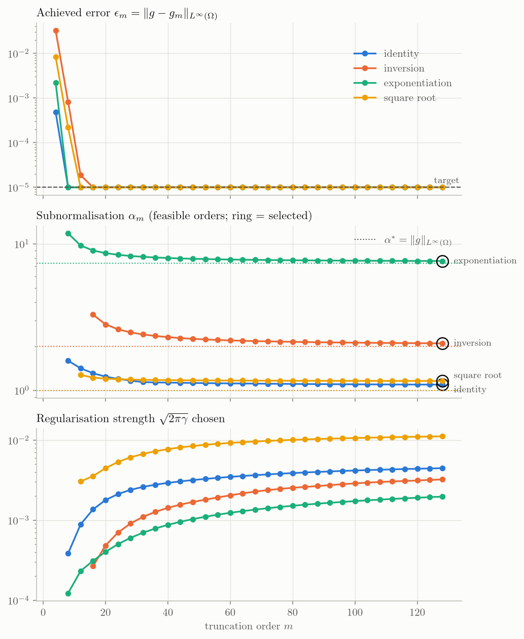
Code: examples/plots/01_error_alpha_vs_m.py

"""
Error, alpha and lambda versus truncation order m
=================================================

Sweep m for each problem at the same target and plot, per m:

- the achieved error eps_m = ||g - g_m||_inf on the fitted set (falls until
  it reaches the target eps_t, then stays there, because the
  regularisation absorbs the remaining slack);
- the subnormalisation alpha_m of each feasible order, against the lower
  bound alpha* = ||g||_inf on the fitted set (dotted), which no fit can beat;
- the regularisation strength lambda = sqrt(2 pi gamma) chosen for it.

The ringed point is the order picked by the default selection
('smallest_alpha').  Needs matplotlib.

Run with:
    python examples/plots/01_error_alpha_vs_m.py [OUTPUT_DIR]
"""

import matplotlib.pyplot as plt
from matplotlib.lines import Line2D

import _style
from felcu import solve_fe_coefficients

TARGET = 1e-5
M_VALUES = range(4, 129, 4)
# Vertical label nudges (points) for the identity and square-root lines, which end close together.
LABEL_DY = {"identity": -5, "square_root": 5}
PROBLEMS = [
    ("identity", dict(sigma_min=-1.0, sigma_max=1.0)),
    ("inversion", dict(sigma_min=0.5, sigma_max=3.0)),
    ("exponentiation", dict(sigma_min=0.1, sigma_max=2.0)),
    ("square_root", dict(sigma_min=0.15, sigma_max=1.0)),
]

_style.apply()
fig, (ax_err, ax_alpha, ax_lam) = plt.subplots(3, 1, sharex=True, figsize=(7, 8.5))

for problem, kwargs in PROBLEMS:
    result = solve_fe_coefficients(problem, target_error=TARGET, m_values=M_VALUES, **kwargs)
    color = _style.PROBLEM_COLORS[problem]
    cands = result.all_results
    feasible = [c for c in cands if c.converged and c.lambda_used > 0]
    alpha_star = _style.alpha_floor(result)

    ax_err.semilogy(
        [c.m for c in cands],
        [c.achieved_linf_error for c in cands],
        marker="o",
        color=color,
        label=_style.PROBLEM_LABELS.get(problem, problem),
    )
    ms, alphas = [c.m for c in feasible], [c.alpha for c in feasible]
    _style.ref_line(ax_alpha, alpha_star, color=color)
    ax_alpha.semilogy(ms, alphas, marker="o", color=color)
    _style.label_end(
        ax_alpha, ms, alphas, _style.PROBLEM_LABELS.get(problem, problem), gap=11, dy=LABEL_DY.get(problem, 0)
    )
    ax_alpha.plot(
        result.m,
        result.alpha,
        marker="o",
        markersize=11,
        markerfacecolor="none",
        markeredgecolor=_style.INK,
        markeredgewidth=1.2,
    )
    ax_lam.semilogy(ms, [c.lambda_used for c in feasible], marker="o", color=color)

    print(f"\n{problem}: selected m={result.m}, alpha={result.alpha:.4f}, alpha* = ||g||_inf = {alpha_star:.4f}")
    print(f"  {'m':>4}  {'Linf':>9}  {'alpha':>9}  {'lambda':>9}")
    for c in cands:
        print(f"  {c.m:>4}  {c.achieved_linf_error:>9.2e}  {c.alpha:>9.4f}  {c.lambda_used:>9.2e}")

_style.target_line(ax_err, TARGET)
ax_err.set_title(r"Achieved error $\epsilon_m = \|g - g_m\|_{L^\infty(\Omega)}$")
ax_err.legend(loc="upper right", bbox_to_anchor=(1, 0.9))
ax_alpha.set_title(r"Subnormalisation $\alpha_m$ (feasible orders; ring = selected)")
ax_alpha.legend(
    handles=[Line2D([], [], color=_style.INK_2, linewidth=1, linestyle=":", label=_style.ALPHA_FLOOR_LABEL)],
    loc="upper right",
)
ax_lam.set_title(r"Regularisation strength $\sqrt{2\pi\gamma}$ chosen")
ax_lam.set_xlabel(r"truncation order $m$")
fig.tight_layout()
_style.finish(fig, "01_error_alpha_vs_m")

The error-alpha trade-off controlled by lambda

At fixed \(m\), felcu chooses the largest regularisation weight \(\gamma\) that still meets the target, so sweeping target_error traces out how \(\epsilon_m\) and \(\alpha_m\) depend on it: more regularisation means a larger error but a smaller \(\alpha_m\), which approaches the lower bound \(\alpha^\ast\) (dotted). Repeated for three orders \(m\).

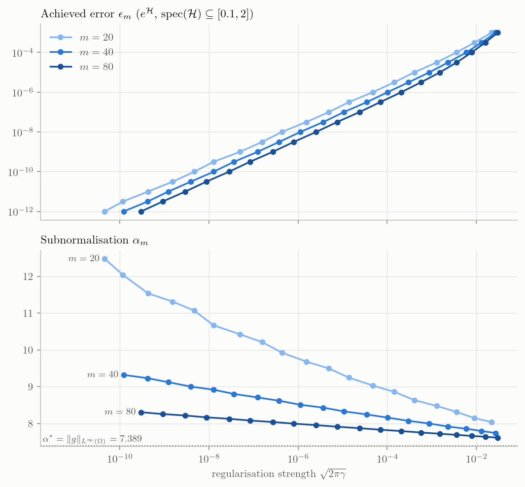
Code: examples/plots/02_error_alpha_vs_lambda.py

"""
The error-alpha trade-off controlled by lambda
==============================================

At fixed m, felcu chooses the largest regularisation weight gamma that
still meets the target eps_t, so sweeping target_error traces out how the
error eps_m and subnormalisation alpha_m depend on lambda = sqrt(2 pi gamma):
more regularisation means a larger error but a smaller alpha_m, which
approaches the lower bound alpha* = ||g||_inf on the fitted set (dotted).
Repeated for three orders m.  Needs matplotlib.

Run with:
    python examples/plots/02_error_alpha_vs_lambda.py [OUTPUT_DIR]
"""

import matplotlib.pyplot as plt
import numpy as np

import _style
from felcu import solve_fe_coefficients

M_ORDERS = (20, 40, 80)
TARGETS = np.geomspace(1e-12, 1e-3, 19)

_style.apply()
fig, (ax_err, ax_alpha) = plt.subplots(2, 1, sharex=True, figsize=(7, 6.5))

for m, color in zip(M_ORDERS, _style.ramp(len(M_ORDERS))):
    rows = []
    for target in TARGETS:
        r = solve_fe_coefficients("exponentiation", sigma_min=0.1, sigma_max=2.0, target_error=target, m=m)
        if r.converged and r.lambda_used > 0:
            rows.append((r.lambda_used, r.achieved_linf_error, r.alpha))
    lam, err, alpha = map(np.array, zip(*rows))

    ax_err.loglog(lam, err, marker="o", color=color, label=f"$m = {m}$")
    ax_alpha.semilogx(lam, alpha, marker="o", color=color)
    _style.label_end(ax_alpha, lam, alpha, f"$m = {m}$", at="start")

    print(f"\nm = {m}")
    print(f"  {'lambda':>9}  {'Linf':>9}  {'alpha':>9}")
    for row in rows:
        print(f"  {row[0]:>9.2e}  {row[1]:>9.2e}  {row[2]:>9.4f}")

alpha_star = _style.alpha_floor(r)
_style.ref_line(ax_alpha, alpha_star, _style.ALPHA_FLOOR_LABEL + f" $= {alpha_star:.3f}$", side="left")
print(f"\nalpha* = ||g||_inf = {alpha_star:.4f}")

ax_alpha.set_xlim(left=ax_alpha.get_xlim()[0] / 10)  # room for the start labels
ax_err.set_title(r"Achieved error $\epsilon_m$  ($e^{\mathcal{H}}$, $\mathrm{spec}(\mathcal{H}) \subseteq [0.1, 2]$)")
ax_err.legend(loc="upper left")
ax_alpha.set_title(r"Subnormalisation $\alpha_m$")
ax_alpha.set_xlabel(r"regularisation strength $\sqrt{2\pi\gamma}$")
fig.tight_layout()
_style.finish(fig, "02_error_alpha_vs_lambda")

Alpha over the Sobolev parameters r and w

The \(H_r^w\) regulariser weights the \(k\)-th Fourier mode by \(P_w(r|k|) = \sum_{j=0}^{w} (r|k|)^{2j}\). At fixed \(m\) and target, sweep \(0 < r \le 1\) and \(w > 1/2\) and plot the resulting subnormalisation \(\alpha_m\), as a heatmap and as slices at four values of \(r\), against the lower bound \(\alpha^\ast\) (dotted). Every fit here meets the target, so only \(\alpha_m\) changes.

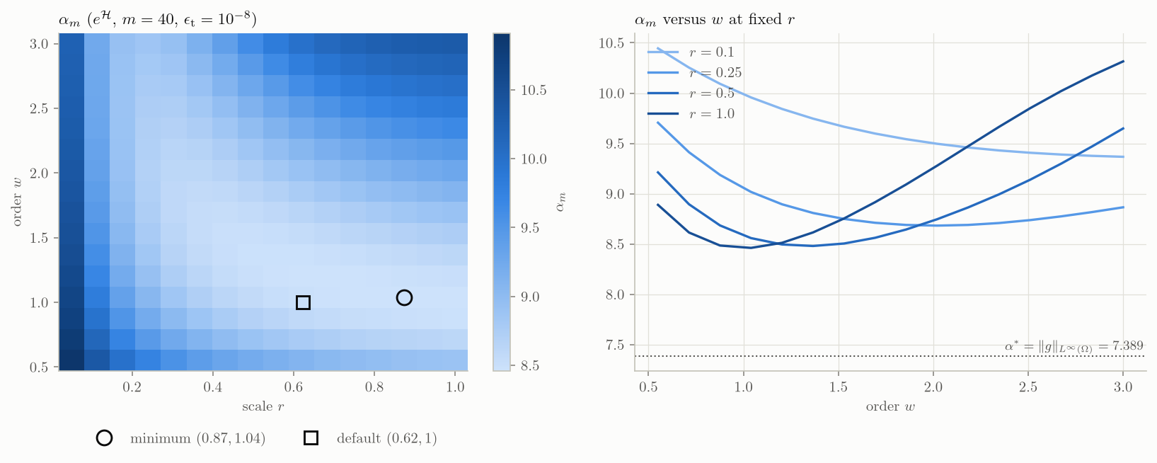
Code: examples/plots/03_alpha_vs_r_w.py

"""
Alpha over the Sobolev parameters r and w
=========================================

The H_r^w regulariser weights the k-th Fourier mode by 1 + (r|k|)^(2w).
At fixed m and target, sweep 0 < r <= 1 and w > 0.5 and plot the resulting
subnormalisation alpha_m, as a heatmap and as slices at four values of r,
against the lower bound alpha* = ||g||_inf on the fitted set (dotted).
Every fit here meets the target, so only alpha_m changes.  Needs matplotlib.

Run with:
    python examples/plots/03_alpha_vs_r_w.py [OUTPUT_DIR]
"""

import matplotlib.pyplot as plt
import numpy as np

import _style
from felcu import solve_fe_coefficients

R = np.linspace(0.05, 1.0, 16)
W = np.linspace(0.55, 3.0, 16)
R_SLICES = (0.1, 0.25, 0.5, 1.0)
common = dict(sigma_min=0.1, sigma_max=2.0, target_error=1e-8, m=40)


def solve(r: float, w: float):
    return solve_fe_coefficients("exponentiation", sobolev_r=r, sobolev_w=w, **common)


grid = np.array([[solve(r, w).alpha for r in R] for w in W])
i, j = np.unravel_index(np.argmin(grid), grid.shape)
default = solve_fe_coefficients("exponentiation", **common)  # r from default_sobolev_r, w = 1
alpha_star = _style.alpha_floor(default)

_style.apply()
fig, (ax_map, ax_cut) = plt.subplots(1, 2, figsize=(11, 4.5))

mesh = ax_map.pcolormesh(R, W, grid, cmap=_style.SEQUENTIAL, shading="nearest")
fig.colorbar(mesh, ax=ax_map, label=r"$\alpha_m$")
ax_map.grid(False)
ax_map.plot(
    R[j],
    W[i],
    marker="o",
    markersize=10,
    markerfacecolor="none",
    markeredgecolor=_style.INK,
    markeredgewidth=1.4,
    linestyle="none",
    label=f"minimum $({R[j]:.2f}, {W[i]:.2f})$",
)
ax_map.plot(
    default.sobolev_r,
    default.sobolev_w,
    marker="s",
    markersize=9,
    markerfacecolor="none",
    markeredgecolor=_style.INK,
    markeredgewidth=1.4,
    linestyle="none",
    label=f"default $({default.sobolev_r:.2f}, {default.sobolev_w:.0f})$",
)
ax_map.legend(loc="upper center", bbox_to_anchor=(0.5, -0.14), ncol=2)
ax_map.set_xlabel(r"scale $r$")
ax_map.set_ylabel(r"order $w$")
ax_map.set_title(r"$\alpha_m$  ($e^{\mathcal{H}}$, $m = 40$, $\epsilon_{\mathrm{t}} = 10^{-8}$)")

for r, color in zip(R_SLICES, _style.ramp(len(R_SLICES))):
    a = [solve(r, w).alpha for w in W]
    ax_cut.plot(W, a, color=color, label=f"$r = {r}$")
_style.ref_line(ax_cut, alpha_star, _style.ALPHA_FLOOR_LABEL + f" $= {alpha_star:.3f}$")
ax_cut.set_xlabel(r"order $w$")
ax_cut.set_title(r"$\alpha_m$ versus $w$ at fixed $r$")
ax_cut.legend(loc="upper left")

fig.tight_layout()

print(f"minimum alpha {grid[i, j]:.4f} at r={R[j]:.3f}, w={W[i]:.3f}")
print(f"default (r={default.sobolev_r:.3f}, w=1) alpha {default.alpha:.4f}")
print(f"alpha* = ||g||_inf = {alpha_star:.4f}")
print("\nalpha  (rows: w, columns: r)")
print("   w \\ r " + " ".join(f"{r:>6.2f}" for r in R[::3]))
for w, row in zip(W[::3], grid[::3]):
    print(f"  {w:>5.2f}  " + " ".join(f"{a:>6.2f}" for a in row[::3]))

_style.finish(fig, "03_alpha_vs_r_w")

Cost of inversion versus condition number

For singular values in \([\kappa^{-1}, 1]\), plot the shortest series that meets the target (selection='smallest_m') and its subnormalisation \(\alpha_m\) as the condition number \(\kappa\) grows. The lower bound \(\alpha^\ast = \|A^{-1}\| = \kappa\) (dotted) is a line rather than a constant.

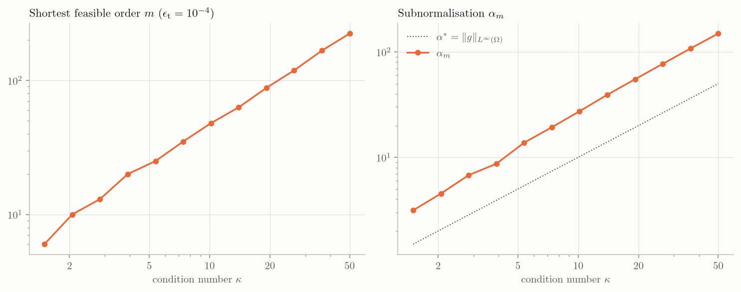
Code: examples/plots/04_inversion_vs_kappa.py

"""
Cost of inversion versus condition number
=========================================

For singular values in [1/kappa, 1], plot the shortest series that meets
the target (selection='smallest_m') and its subnormalisation alpha_m as the
condition number kappa grows.  The lower bound alpha* = ||g||_inf on the
fitted set (dotted) equals ||A^-1|| = kappa here, so it is a line rather
than a constant.
Needs matplotlib.

Run with:
    python examples/plots/04_inversion_vs_kappa.py [OUTPUT_DIR]
"""

import matplotlib.pyplot as plt
import numpy as np
from matplotlib.ticker import NullFormatter

import _style
from felcu import solve_fe_coefficients

TARGET = 1e-4
KAPPAS = np.geomspace(1.5, 50, 12)
color = _style.PROBLEM_COLORS["inversion"]

rows = []
for kappa in KAPPAS:
    r = solve_fe_coefficients(
        "inversion",
        sigma_min=1.0 / kappa,
        sigma_max=1.0,
        spectral_kind="singular_values",
        target_error=TARGET,
        selection="smallest_m",
    )
    rows.append((kappa, r.m, r.alpha, _style.alpha_floor(r), r.converged))

kappa, m, alpha, alpha_star, conv = map(np.array, zip(*rows))
ok = conv.astype(bool)

_style.apply()
fig, (ax_m, ax_alpha) = plt.subplots(1, 2, figsize=(10, 4))
ax_m.loglog(kappa[ok], m[ok], marker="o", color=color)
ax_m.set_title(r"Shortest feasible order $m$  ($\epsilon_{\mathrm{t}} = 10^{-4}$)")
ax_alpha.loglog(kappa, alpha_star, color=_style.INK_2, linewidth=1, linestyle=":", label=_style.ALPHA_FLOOR_LABEL)
ax_alpha.loglog(kappa[ok], alpha[ok], marker="o", color=color, label=r"$\alpha_m$")
ax_alpha.legend(loc="upper left")
ax_alpha.set_title(r"Subnormalisation $\alpha_m$")
for ax in (ax_m, ax_alpha):
    ax.set_xlabel(r"condition number $\kappa$")
    ax.set_xticks([2, 5, 10, 20, 50], labels=["$2$", "$5$", "$10$", "$20$", "$50$"])
    ax.xaxis.set_minor_formatter(NullFormatter())
fig.tight_layout()

print(f"{'kappa':>7}  {'m':>4}  {'alpha':>9}  {'alpha*':>9}  converged")
for row in rows:
    print(f"{row[0]:>7.2f}  {row[1]:>4}  {row[2]:>9.3f}  {row[3]:>9.3f}  {row[4]}")
if not ok.all():
    print("\n(non-converged points are left out of the plot: increase m_values to reach them)")

_style.finish(fig, "04_inversion_vs_kappa")

The fitted series over a whole period, and its pointwise error

Top: the series \(g_m\) over the full period \(\mathbb T = [-\pi, \pi)\) against the target \(g\) on the fitted set \(\Omega\). The shaded regions are not fitted: the extension region, and for indefinite inversion also the gap around the pole, where \(g_m\) stays bounded. Bottom: \(|g - g_m|\) on \(\Omega\).

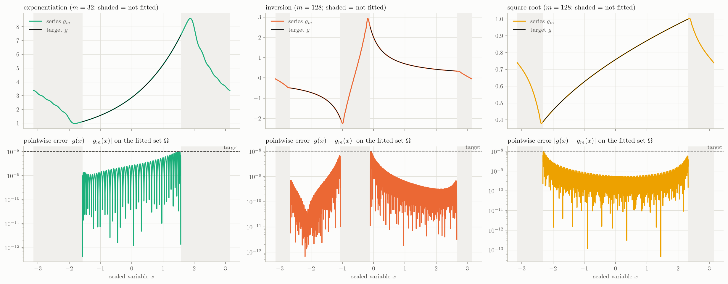
Code: examples/plots/05_pointwise_error.py

"""
The fitted series over a whole period, and its pointwise error
==============================================================

Top: the series g_m over the full period [-pi, pi] against the target g on
the fitted set Omega.  The shaded regions are not fitted: the extension
region, and for indefinite inversion also the gap around the pole, where
g_m stays bounded.  Bottom: |g - g_m| on Omega.  Needs matplotlib.

Run with:
    python examples/plots/05_pointwise_error.py [OUTPUT_DIR]
"""

import matplotlib.pyplot as plt
import numpy as np

import _style
from felcu import (
    evaluate_fourier_series,
    evaluate_target_function,
    fitted_domain_segments,
    solve_fe_coefficients,
)

TARGET = 1e-8
CASES = [
    ("exponentiation", dict(sigma_min=0.1, sigma_max=2.0, m_values=range(4, 33, 2))),
    ("inversion", dict(sigma_min=-2.0, sigma_max=3.0, gap=(-0.5, 0.4), m_values=range(8, 129, 8))),
    ("square_root", dict(sigma_min=0.15, sigma_max=1.0, m_values=range(8, 129, 8))),
]

_style.apply()
fig, axes = plt.subplots(2, len(CASES), figsize=(5.5 * len(CASES), 6.5), sharex=True)
x_full = np.linspace(-np.pi, np.pi, 2001)

for col, (problem, kwargs) in enumerate(CASES):
    r = solve_fe_coefficients(problem, target_error=TARGET, **kwargs)
    color = _style.PROBLEM_COLORS[problem]
    ax_fit, ax_err = axes[0, col], axes[1, col]
    segments = fitted_domain_segments(r)

    # Shade everything outside the fitted segments
    edges = [-np.pi] + [v for s in segments for v in (s[0], s[-1])] + [np.pi]
    for ax in (ax_fit, ax_err):
        for left, right in zip(edges[::2], edges[1::2]):
            ax.axvspan(left, right, color=_style.SHADE, linewidth=0)

    g = evaluate_fourier_series(x_full, r.a0, r.ak, r.bk)
    ax_fit.plot(x_full, g, color=color, label="series $g_m$")
    worst = 0.0
    for i, xs in enumerate(segments):
        f = evaluate_target_function(xs, r)
        err = np.abs(evaluate_fourier_series(xs, r.a0, r.ak, r.bk) - f)
        worst = max(worst, err.max())
        ax_fit.plot(xs, f, color=_style.INK, linewidth=0.9, label="target $g$" if i == 0 else None)
        ax_err.semilogy(xs, err, color=color)

    _style.target_line(ax_err, TARGET)
    ax_fit.set_title(f"{_style.PROBLEM_LABELS.get(problem, problem)}  ($m = {r.m}$; shaded = not fitted)")
    ax_fit.legend(loc="upper left")
    ax_err.set_title(r"pointwise error $|g(x) - g_m(x)|$ on the fitted set $\Omega$")
    ax_err.set_xlabel(r"scaled variable $x$")
    print(f"{problem}: m={r.m}  x_gap={r.x_gap}  max |g - f| = {worst:.2e}  (target {TARGET:g})")

fig.tight_layout()
_style.finish(fig, "05_pointwise_error")

Cost of the square root versus condition number

For eigenvalues in \([\kappa^{-1}, 1]\), fit \(\sqrt{\mathcal H}\) (with the default \(\eta_{\rm def}\) and \(r_{\rm sqrt} = \kappa^{-1/2}\)) and plot the shortest series that meets the target and the smallest subnormalisation \(\alpha_m\) over the sweep as \(\kappa\) grows. \(\|\sqrt{\mathcal H}\| = 1\) throughout, so the lower bound \(\alpha^\ast = 1\) (dotted) is constant. Unlike inversion, \(\sqrt x\) is concave and the periodic closure narrows with \(\kappa\), so the paper predicts \(\alpha_m = O(\kappa^{1/4})\) for \(w = 1\) (dashed); over this range the growth stays below that rate.

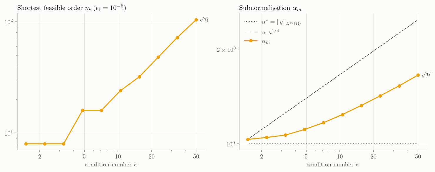
Code: examples/plots/06_sqrt_vs_kappa.py

"""
Cost of the square root versus condition number
===============================================

For eigenvalues in [1/kappa, 1], fit sqrt(H) (with the default
eta_def and r_sqrt = kappa^(-1/2)) and plot the shortest series that meets
the target and the smallest subnormalisation alpha_m over the sweep as
kappa grows.  ||sqrt(H)|| = 1 throughout, so the
lower bound alpha* = 1 (dotted) is constant.  Unlike inversion, sqrt is
concave and the periodic closure narrows with kappa, so the paper predicts
alpha_m = O(kappa^(1/4)) for w = 1 (dashed, through the first point).
Needs matplotlib.

Run with:
    python examples/plots/06_sqrt_vs_kappa.py [OUTPUT_DIR]
"""

import matplotlib.pyplot as plt
import numpy as np
from matplotlib.ticker import NullFormatter

import _style
from felcu import solve_fe_coefficients

TARGET = 1e-6
KAPPAS = np.geomspace(1.5, 50, 10)
color = _style.PROBLEM_COLORS["square_root"]

rows = []
for kappa in KAPPAS:
    r = solve_fe_coefficients(
        "square_root",
        sigma_min=1.0 / kappa,
        sigma_max=1.0,
        target_error=TARGET,
        m_values=range(8, 257, 8),
    )
    m_min = min((c.m for c in r.all_results if c.converged), default=0)
    rows.append((kappa, m_min, r.alpha, _style.alpha_floor(r), r.converged))

kappa, m, alpha, alpha_star, conv = map(np.array, zip(*rows))
ok = conv.astype(bool)

_style.apply()
fig, (ax_m, ax_alpha) = plt.subplots(1, 2, figsize=(10, 4))
ax_m.loglog(kappa[ok], m[ok], marker="o", color=color)
_style.label_end(ax_m, kappa[ok], m[ok], r"$\sqrt{\mathcal{H}}$")
ax_m.set_title(r"Shortest feasible order $m$  ($\epsilon_{\mathrm{t}} = 10^{-6}$)")
ax_alpha.loglog(kappa, alpha_star, color=_style.INK_2, linewidth=1, linestyle=":", label=_style.ALPHA_FLOOR_LABEL)
first = np.argmax(ok)
ax_alpha.loglog(
    kappa,
    alpha[first] * (kappa / kappa[first]) ** 0.25,
    color=_style.INK_2,
    linewidth=1,
    linestyle="--",
    label=r"$\propto \kappa^{1/4}$",
)
ax_alpha.loglog(kappa[ok], alpha[ok], marker="o", color=color, label=r"$\alpha_m$")
_style.label_end(ax_alpha, kappa[ok], alpha[ok], r"$\sqrt{\mathcal{H}}$")
ax_alpha.legend(loc="upper left")
ax_alpha.set_title(r"Subnormalisation $\alpha_m$")
for ax in (ax_m, ax_alpha):
    ax.set_xlabel(r"condition number $\kappa$")
    ax.set_xticks([2, 5, 10, 20, 50], labels=["$2$", "$5$", "$10$", "$20$", "$50$"])
    ax.xaxis.set_minor_formatter(NullFormatter())
fig.tight_layout()

print(f"{'kappa':>7}  {'m_min':>5}  {'alpha':>9}  {'alpha*':>9}  converged")
for row in rows:
    print(f"{row[0]:>7.2f}  {row[1]:>5}  {row[2]:>9.3f}  {row[3]:>9.3f}  {row[4]}")
if not ok.all():
    print("\n(non-converged points are left out of the plot: increase m_values to reach them)")

_style.finish(fig, "06_sqrt_vs_kappa")

Comparing the three coefficient-selection methods

The paper's numerical comparison: the identity, exponential, square root and inverse, each fitted by the reflected extension (refl), arcsine-Taylor (asin) and the Sobolev-regularised extension (reg); see Method. Arcsine-Taylor uses \(\eta = 3\) for the entire functions, and \(\eta = 2.7\) and \(2.5\) for the square root and inverse, just below their analyticity bounds \(2\mu/\delta\).

• Top: each series \(g_m\) for \(m = 128\) over one whole period, mapped back to the eigenvalue \(\lambda = \mu + x/\tau\) so that all three share the target \(f\) on the spectral interval (unshaded). Each method's period is set by its own \(\eta\), and outside the spectrum they extend \(f\) differently: the reflected extension mirrors it, while arcsine-Taylor follows \(f\) out to \(\mu \pm \eta\delta/2\) before turning back.
• Middle: the error \(\epsilon_m\). The reflected extension converges as \(O(m^{-1})\), arcsine-Taylor exponentially with factor \(\sin(\pi/\eta)\), and the regularised fit drops straight to the target.
• Bottom: \(\alpha_m\), against the lower bound \(\alpha^\ast\) (dotted). The reflected extension sits on it for the convex functions, \(\alpha_m = \|f(\mathcal H)\| - \epsilon_m\). For those functions arcsine-Taylor approaches the larger limit \(|f(\mu \pm \eta\delta/2)|\) (dashed). The regularised \(\alpha_m\) is shown for the orders that meet the target, and falls towards \(\alpha^\ast\).

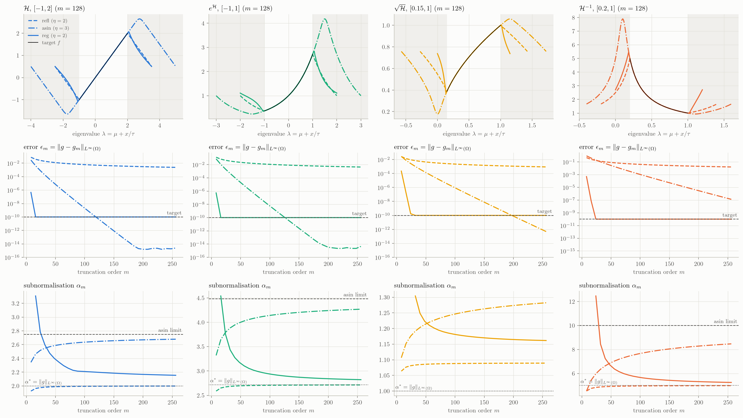
Code: examples/plots/07_method_comparison.py

"""
Comparing the three coefficient-selection methods
=================================================

The paper's numerical comparison (its Fig. 1): the identity, exponential,
square root and inverse, each fitted by the reflected extension ("refl"),
arcsine-Taylor ("asin") and the Sobolev-regularised extension ("reg").

Top: each series g_m for m = 128 over one whole period, mapped back to the
eigenvalue lambda = mu + x / tau so that all three share the target f, which
is drawn on the spectral interval (unshaded).  The methods agree there but
extend f differently outside it, over periods set by their own eta.
Middle: the error eps_m against m.  Bottom: alpha_m against m, with the
lower bound alpha* = ||f(H)|| (dotted) and, for the convex functions, the
arcsine-Taylor limit |f(mu +- eta delta / 2)| (dashed).  The reflected
extension sits just below alpha* but converges as O(1/m); arcsine-Taylor
converges exponentially towards a larger alpha; the regularised fit reaches
the target with alpha close to alpha*.  Sobolev alpha is shown for the
orders that meet the target.  Needs matplotlib.

Run with:
    python examples/plots/07_method_comparison.py [OUTPUT_DIR]
"""

import warnings

import matplotlib.pyplot as plt
import numpy as np

import _style
from felcu import ConvergenceWarning, evaluate_fourier_series, solve_fe_coefficients

# The reflected method converges only like O(1/m), so it never reaches TARGET;
# the plot is there to show that.
warnings.simplefilter("ignore", ConvergenceWarning)

TARGET = 1e-10
M_VALUES = range(8, 257, 8)
M_SHOW = 128

# (problem, f, spectral interval, arcsine-Taylor eta, f convex).  eta = 3 for
# the entire functions; the others sit below their analyticity bounds
# 2 mu / delta, 46/17 ~ 2.71 for the square root and 3 for the inverse, as in
# the paper.  The arcsine-Taylor limit of alpha only holds for convex f.
CASES = [
    ("identity", r"$\mathcal{H}$", lambda t: t, (-1.0, 2.0), 3.0, True),
    ("exponentiation", r"$e^{\mathcal{H}}$", np.exp, (-1.0, 1.0), 3.0, True),
    ("square_root", r"$\sqrt{\mathcal{H}}$", np.sqrt, (0.15, 1.0), 2.7, False),
    ("inversion", r"$\mathcal{H}^{-1}$", lambda t: 1.0 / t, (0.2, 1.0), 2.5, True),
]
METHODS = {
    "reflected": ("refl", "--"),
    "arcsine_taylor": ("asin", "-."),
    "sobolev": ("reg", "-"),
}

_style.apply()
fig, axes = plt.subplots(3, len(CASES), figsize=(4.2 * len(CASES), 9.5))
x_full = np.linspace(-np.pi, np.pi, 2001)

print(f"{'problem':<15} {'method':<15} {'eta':>5}  {'eps_128':>9}  {'alpha_128':>9}  {'alpha*':>9}")
for col, (problem, name, f, (lo, hi), eta_asin, convex) in enumerate(CASES):
    color = _style.PROBLEM_COLORS[problem]
    ax_fit, ax_err, ax_alpha = axes[:, col]
    mu, delta = (lo + hi) / 2, (hi - lo) / 2
    common = dict(sigma_min=lo, sigma_max=hi, target_error=TARGET, m_values=M_VALUES)

    for method, (short, linestyle) in METHODS.items():
        kwargs = common | ({"eta": eta_asin} if method == "arcsine_taylor" else {})
        r = solve_fe_coefficients(problem, method=method, **kwargs)
        sweep = r.all_results
        shown = next(c for c in sweep if c.m == M_SHOW)
        style = dict(color=color, linestyle=linestyle, label=f"{short} ($\\eta = {r.eta:.3g}$)")

        # Each method scales the spectrum by its own tau, so compare in lambda.
        lam = mu + x_full / shown.tau
        ax_fit.plot(lam, evaluate_fourier_series(x_full, shown.a0, shown.ak, shown.bk), **style)
        ax_err.semilogy([c.m for c in sweep], [c.achieved_linf_error for c in sweep], **style)
        keep = [c for c in sweep if method != "sobolev" or c.converged]
        ax_alpha.plot([c.m for c in keep], [c.alpha for c in keep], **style)
        print(
            f"{problem:<15} {method:<15} {r.eta:>5.3g}  {shown.achieved_linf_error:>9.1e}  "
            f"{shown.alpha:>9.4f}  {_style.alpha_floor(r):>9.4f}"
        )

    left, right = ax_fit.get_xlim()
    ax_fit.axvspan(left, lo, color=_style.SHADE, linewidth=0, zorder=0)
    ax_fit.axvspan(hi, right, color=_style.SHADE, linewidth=0, zorder=0)
    ax_fit.set_xlim(left, right)
    spectrum = np.linspace(lo, hi, 201)
    ax_fit.plot(spectrum, f(spectrum), color=_style.INK, linewidth=0.9, label="target $f$")

    _style.target_line(ax_err, TARGET)
    _style.ref_line(ax_alpha, _style.alpha_floor(r), _style.ALPHA_FLOOR_LABEL, side="left")
    if convex:
        asin_limit = max(abs(f(mu - eta_asin * delta / 2)), abs(f(mu + eta_asin * delta / 2)))
        _style.ref_line(ax_alpha, asin_limit, "asin limit", linestyle="--")

    ax_fit.set_title(f"{name}, $[{lo:g}, {hi:g}]$  ($m = {M_SHOW}$)")
    ax_fit.set_xlabel(r"eigenvalue $\lambda = \mu + x/\tau$")
    ax_err.set_title(r"error $\epsilon_m = \|g - g_m\|_{L^\infty(\Omega)}$")
    ax_err.set_ylim(1e-16, None)
    ax_alpha.set_title(r"subnormalisation $\alpha_m$")
    for ax in (ax_err, ax_alpha):
        ax.set_xlabel("truncation order $m$")
    if col == 0:
        ax_fit.legend(loc="upper left", fontsize=8)

fig.tight_layout()
_style.finish(fig, "07_method_comparison")